
In this article, we’ll investigate whether it’s possible to significantly improve the recovery factor of an EA (Expert Advisor) with a 50% win rate by adjusting lot sizes using the Decomposition Monte Carlo Method. We’ll then delve into the results and consider their implications.
Please follow along with the discussion outlined below:
- We’ll prepare an EA with a win rate of approximately 50% over a period of 10 years.
- We’ll try out several methods for adjusting the lot sizes.
- We’ll check to what extent the recovery factor improves.
Understanding the Recovery Factor
The recovery factor is a metric used in backtesting an EA, serving as one of the indicators for evaluating a trading strategy’s performance. It represents the ratio between the profit obtained and the drawdown (temporary loss). The calculation formula is as follows:
The Base Model EA with 50% Win Rate
Firstly, we’ll prepare an Expert Advisor (EA) with approximately a 50% win rate.
Trading Strategy
The trading strategy of this base model EA is as follows (It’s a non-Martingale EA):
- We determine the timing of buying and selling using technical indicators such as Moving Average (MA) and Directional Movement Index (DMI).
- The Take Profit and Stop Loss levels are set based on the Average True Range (ATR).
- We have set the Take Profit and Stop Loss levels to be nearly the same, but we have made the Take Profit slightly larger so that the profit and loss can be positive even with a 50% win rate.
- We will take up to four positions simultaneously for both buy and sell positions, but each position will independently carry out profit-taking and stop-loss. (This is not a Martingale strategy, but rather imagine four separate trading strategies running concurrently.)
The performance of this base model is as follows:
Backtesting Setup
| Asset: | GBPJPY | |||||||||||
| Duration: | 10 years (01.01.2013 – 12.31.2022) | |||||||||||
| Currency: | USD | |||||||||||
| Initial Margin: | 10,000 USD | |||||||||||
| Lot Size: | Fixed at 0.01 | |||||||||||
Backtesting Results
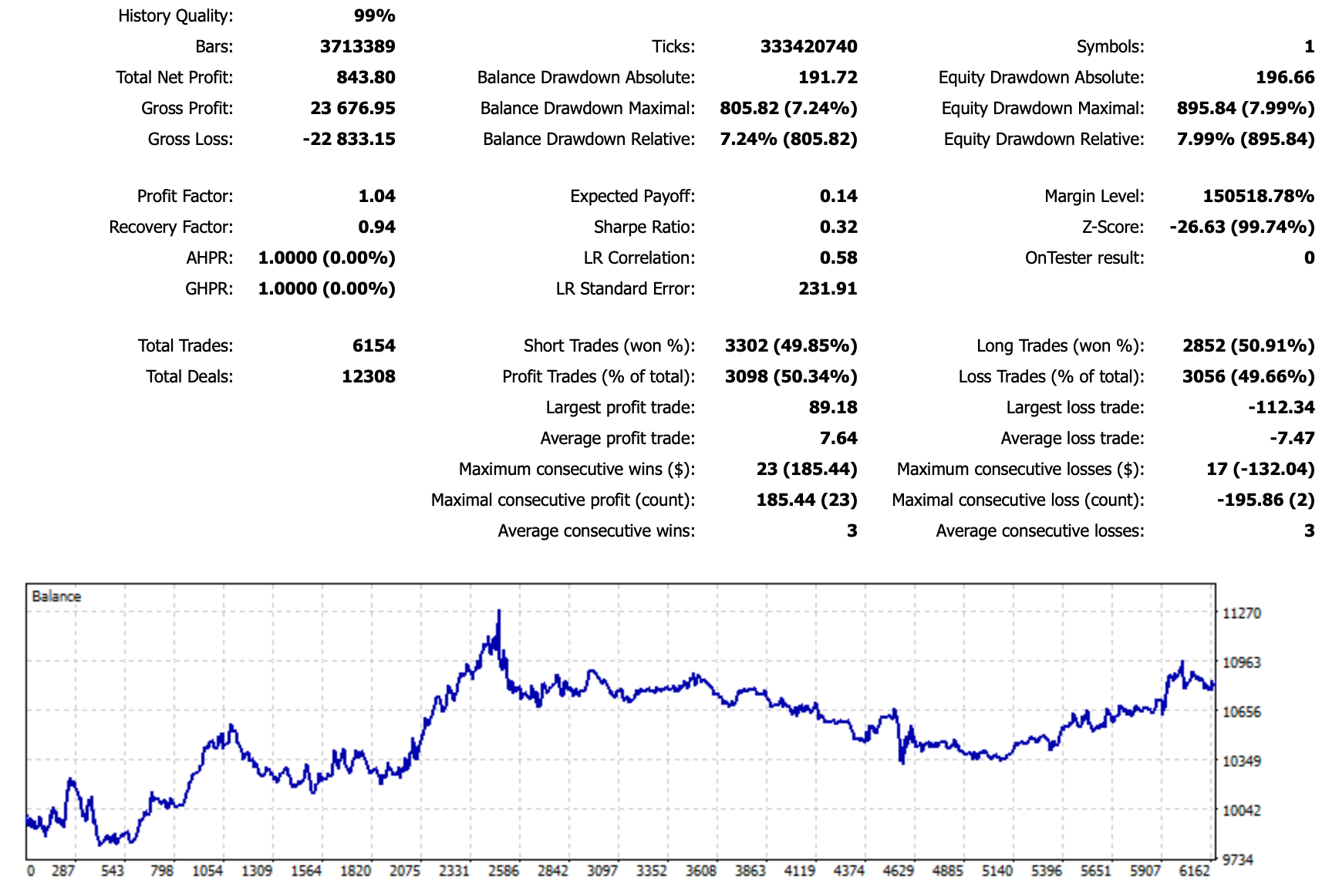
Performance Analysis
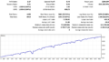
- Over a span of 10 years, Total Net Profit was 843.80 USD.
- Equity Drawdown Maximal was 895.84 USD.
- Total Trades was 6,154, with a win rate of 50.34%.
- Profit Factor was 1.04, and Recovery Factor was 0.94.
As you can see from the chart, over a decade, the win rate is approximately 50%. Therefore, there are periods of continuous wins and losses, and depending on how the period is segmented, the performance may fall below 50%. The goal of this test is to optimize the shape of this chart as much as possible just by adjusting the lot size.
Setting the Lot Size
In the base model, the lot size is fixed at 0.01. In other words, while there are 6,154 trades in the backtest, all these trades were conducted with a lot size of 0.01.
In the following strategies, we will only change this lot size setting and verify how the backtest results change.
Introduction of the Martingale Method (No Lot Size Limit)
First, let’s test the introduction of the Martingale method to the lot size setting.
In this case, we’ll apply the Martingale method by considering each trade to end either in profit-taking or a stop-loss. We’ll define a trade that ends in profit-taking as a win and one that ends in a stop-loss as a loss.
Reviewing the Rules for Determining Lot Size
In the Martingale strategy, where the lot size is doubled after a loss, the position size (lot size) is increased twofold each time a continuous stop loss occurs. Consider the following scenario if the initial lot size is 0.01:
- 1st trade: Lot size 0.01 (Stop loss)
- 2nd trade: Lot size 0.02 (Stop loss)
- 3rd trade: Lot size 0.04 (Stop loss)
- 4th trade: Lot size 0.08 (Stop loss)
- 5th trade: Lot size 0.16 (Stop loss)
- 6th trade: Lot size 0.32 (Profit taken)
In this example, there are five consecutive stop losses before a profit is taken on the sixth trade. The total lot size of the losing trades is 0.31. However, since the lot size of the sixth trade is 0.32, if a profit is taken, you can recover the losses from the previous stop losses and earn a profit equivalent to a lot size of 0.01.
Furthermore, as you will see if you actually check, no matter which trade results in a win (profit taken), the final profit will be equivalent to a lot size of 0.01. This is an example of the Martingale strategy with a Martingale ratio of 2x.
By the way, the rule is to start again from 0.01 for the next trade once a profit is taken. The risk is high as the lot size will continue to increase infinitely if losses continue, but for now, we will test without setting a limit on the lot size.
Backtesting Setup
| Asset: | GBPJPY | |||||||||||
| Duration: | 10 years (01.01.2013 – 12.31.2022) | |||||||||||
| Currency: | USD | |||||||||||
| Initial Margin: | 1,000,000 USD | |||||||||||
| Lot Size: | Martingale Method (No Lot Size Limit) | |||||||||||
Backtesting Results
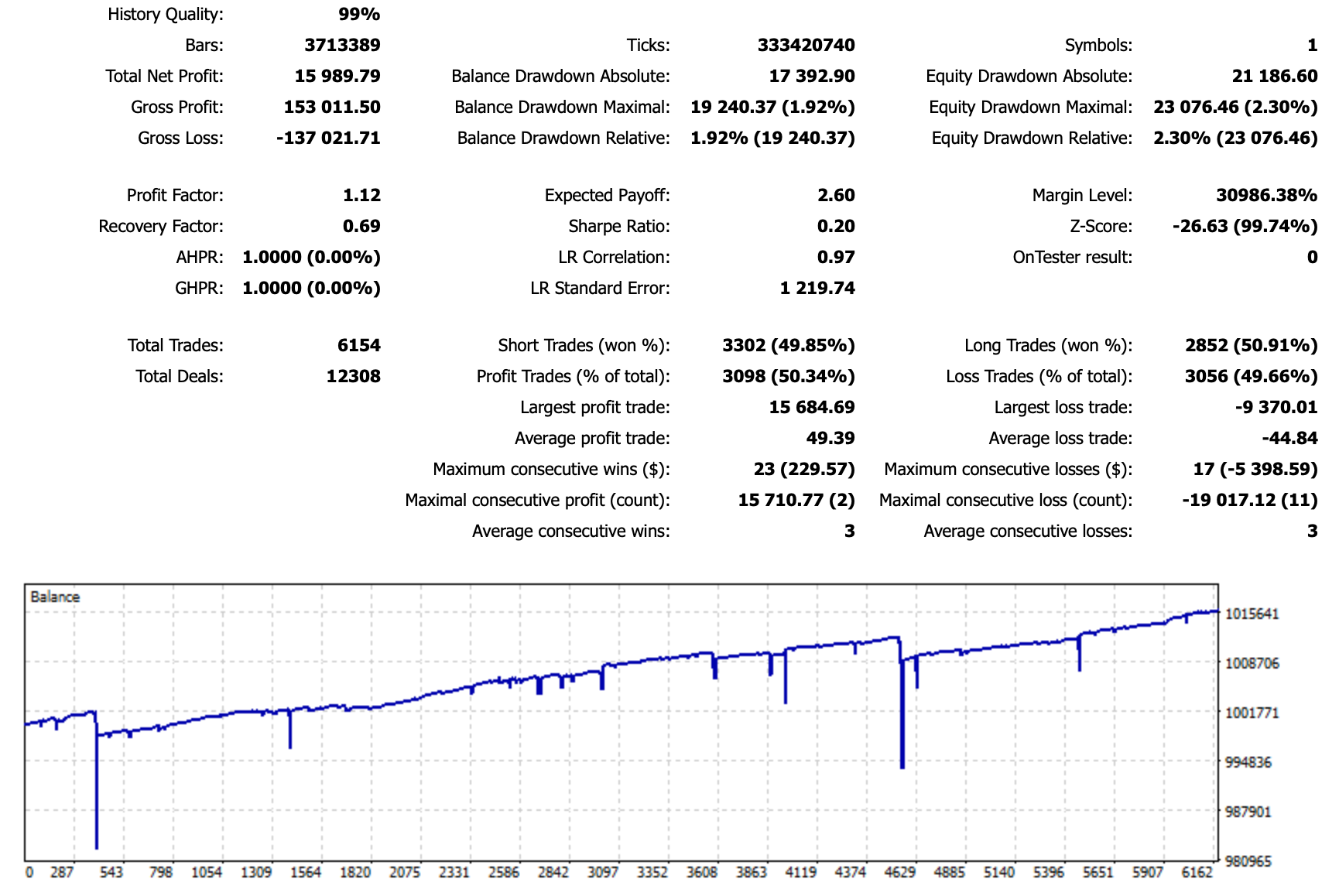
Performance Analysis
- Over a span of 10 years, Total Net Profit was 15,989.79 USD.
- Equity Drawdown Maximal was 23,076.46 USD.
- Total Trades was 6,154, with a win rate of 50.34% (exactly the same as the base model).
- Profit Factor was 1.12, and Recovery Factor was 0.69.
While a profit of 15 thousand dollars can be made over ten years, the maximum drawdown is 23 thousand dollars, which means the recovery factor falls below 0.70. This implies that while the absolute amount of profit has increased, the amount of margin required to avoid bankruptcy has also increased, leading to a decline in capital efficiency.
It’s important to note here that the number of trades and the win rate are exactly the same as the previous base model. Even if the trade timing is exactly the same, changing only the lot size strategy can result in significantly different outcomes. This should be quite clear.
This kind of graph is common in EAs that incorporate the Martingale strategy. Because this strategy always recoups losses if there is an infinite amount of funds, the profit and loss graph tends to have an upward trend.
Introducing the Martingale Method (With a Lot Size Limit)
Next, let’s consider a model that adds a lot size limit to the Martingale method.
Backtesting Setup
| Asset: | GBPJPY | |||||||||||
| Duration: | 10 years (01.01.2013 – 12.31.2022) | |||||||||||
| Currency: | USD | |||||||||||
| Initial Margin: | 10,000 USD | |||||||||||
| Lot Size: | Martingale Method (Maximum Lot Size 0.30) | |||||||||||
For this, we’ll return the initial margin to 1 million yen, and set the maximum lot size to 0.30.
Backtesting Results
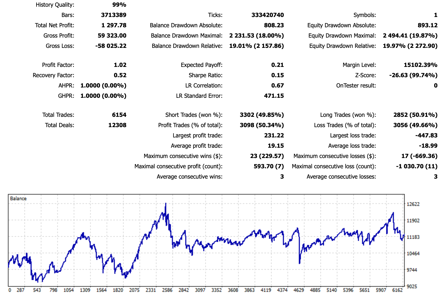
Performance Analysis
- Over a span of 10 years, Total Net Profit was 1,297.78 USD.
- Equity Drawdown Maximal was 2,494.41 USD.
- Total Trades was 6,154, with a win rate of 50.34% (exactly the same as the base model).
- Profit Factor was 1.02, and Recovery Factor was 0.56.
By imposing a limit on the number of lots, both profits and drawdowns have decreased to about one-tenth. However, the recovery factor has further deteriorated. It is evident that setting the maximum number of lots limit to 0.30 (5 consecutive losses) has not been effective. Even with a 50% winning rate, it seems that about 5 consecutive losses occur quite frequently.
Calculating probabilities, the chance of experiencing a 50% (1/2) loss five times in a row is about 3%. However, if there are 6,000 transactions, it would occur 180 times, which does not seem to be such a rare occurrence.
In conclusion, it is quite difficult to improve the recovery factor using the Martingale method.
Introduction of Decomposition Monte Carlo Method (with lot size limit)
Next, we will examine the decomposition Monte Carlo method.
With the application to EA in mind, the features of this decomposed Monte Carlo method can be briefly summarized as follows:
- When the number sequence is reset, the final balance becomes positive.
- The increase in the number of lots is gradual, and losses are recovered slowly over time.
- Based on these points, it can be said that this is an improved version of the Martingale method that reduces risk.
Confirming the rules for determining the number of lots
Rules of the number sequence
- First, prepare a number sequence of [0, 1].
- Bet the sum of the numbers at the left and right ends of the number sequence. (Initially 0+1=1)
- If you lose: Add the bet amount to the right end of the number sequence
- If you win: Erase the numbers at the far right and far left of the number sequence
- If the number sequence completely disappears, reset the number sequence. The sequence starts again from [0, 1].
- If one number remains in the sequence, decompose the number as evenly as possible. The sequence will use the two decomposed numbers arranged in a sequence.
For example: When decomposing numbers, write the smaller number on the left and the larger number on the right. “5→[2, 3]”, “8→[4, 4]”, “11→[5, 6]”
Deciding Lot Size Rule
We use the lot size of 0.01 times the bet derived from the above sequence of rules in trading.
To better understand the rule, let’s compute the lot size in case of losing thrice, winning once, losing four times, and then winning four times. (Bear with us as this might be a bit lengthy, but it would be easier to understand the rule with a concrete example.)
- 1st Trade
- Sequence: [0, 1] (initial sequence)
- Lot Size: 0.01 (0+1=1)
- Result: Stop Loss
- 2nd Trade
- Sequence: [0, 1, 1] (since we lost the previous round, add 1 to the right end)
- Lot Size: 0.01 (0+1=1)
- Result: Stop Loss
- 3rd Trade
- Sequence: [0, 1, 1, 1] (since we lost the previous round, add 1 to the right end)
- Lot Size: 0.01 (0+1=1)
- Result: Stop Loss
- 4th Trade
- Sequence: [0, 1, 1, 1, 1] (since we lost the previous round, add 1 to the right end)
- Lot Size: 0.01 (0+1=1)
- Result: Take Profit
- 5th Trade
- Sequence: [1, 1, 1] (since we won the previous round, remove numbers from both ends)
- Lot Size: 0.02 (1+1=2)
- Result: Stop Loss
- 6th Trade
- Sequence: [1, 1, 1, 2] (since we lost the previous round, add 2 to the right end)
- Lot Size: 0.03 (1+2=3)
- Result: Stop Loss
- 7th Trade
- Sequence: [1, 1, 1, 2, 3] (since we lost the previous round, add 3 to the right end)
- Lot Size: 0.04 (1+3=4)
- Result: Stop Loss
- 8th Trade
- Sequence: [1, 1, 1, 2, 3, 4] (since we lost the previous round, add 4 to the right end)
- Lot Size: 0.05 (1+4=5)
- Result: Stop Loss
- 9th Trade
- Sequence: [1, 1, 1, 2, 3, 4, 5] (since we lost the previous round, add 5 to the right end)
- Lot Size: 0.06 (1+5=6)
- Result: Take Profit
- 10th Trade
- Sequence: [1, 1, 2, 3, 4] (since we won the previous round, remove numbers from both ends)
- Lot Size: 0.05 (1+4=5)
- Result: Take Profit
- 11th Trade
- Sequence: [1, 2, 3] (since we won the previous round, remove numbers from both ends)
- Lot Size: 0.04 (1+3=4)
- Result: Take Profit
- 12th Trade
- Sequence: [2] (since we won the previous round, remove numbers from both ends)
- Sequence: [1, 1] (since we only have one number left, we decompose 2)
- Lot Size: 0.02 (1+1=2)
- Result: Take Profit (Once all numbers are gone, the sequence is over.)
To summarize the results in a tabular form, here’s what we have:
| Round | Sequence | Lot Size | Result |
|---|---|---|---|
| 1 | [0, 1] | 0.01 | Stop Loss |
| 2 | [0, 1, 1] | 0.01 | Stop Loss |
| 3 | [0, 1, 1, 1] | 0.01 | Stop Loss |
| 4 | [0, 1, 1, 1, 1] | 0.01 | Take Profit |
| 5 | [1, 1, 1] | 0.02 | Stop Loss |
| 6 | [1, 1, 1, 2] | 0.03 | Stop Loss |
| 7 | [1, 1, 1, 2, 3] | 0.04 | Stop Loss |
| 8 | [1, 1, 1, 2, 3, 4] | 0.05 | Stop Loss |
| 9 | [1, 1, 1, 2, 3, 4, 5] | 0.06 | Take Profit |
| 10 | [1, 1, 2, 3, 4] | 0.05 | Take Profit |
| 11 | [1, 2, 3] | 0.04 | Take Profit |
| 12 | [1, 1] | 0.02 | Take Profit |
From the above, the total lot size for stop loss is 0.17, and the total lot size for taking profit is 0.18. This means that we can secure a profit of 0.01 in lot size and conclude the set.
In this series of operations, we can see that even when we lose, the lot size does not increase, or it only increases by 0.01. In contrast to the Martingale method where the lot size doubles, the increase in lot size in the Fractional Monte Carlo method is gradual. Moreover, while in the Martingale method a single win concludes a set, in the Fractional Monte Carlo method, it takes five wins to end a set. Therefore, the process of recovering losses is also gradual.
Backtesting Setup
| Asset: | GBPJPY | |||||||||||
| Duration: | 10 years (01.01.2013 – 12.31.2022) | |||||||||||
| Currency: | USD | |||||||||||
| Initial Margin: | 10,000 USD | |||||||||||
| Lot Size: | Decomposition Monte Carlo Method (Maximum Lot Size 0.30) | |||||||||||
Backtesting Results

Performance Analysis
- Over a span of 10 years, Total Net Profit was 6,811.63 USD.
- Equity Drawdown Maximal was 2,382.97 USD.
- Total Trades was 6,154, with a win rate of 50.34% (exactly the same as the base model).
- Profit Factor was 1.13, and Recovery Factor was 2.86.
The recovery factor has improved to about three times that of the base model. The upward trend of the graph is visually clear, and we can see that significant drawdowns have become less frequent.
Conclusion
In this article, I’ve shared the backtest results of four different Expert Advisors (EAs), all of which had the exact same number of trades at 6,154 and win rates of 50.34%. Please take note of this.
In other words, all four EAs entered and exited trades at the same time, with the same win-loss ratio. The only difference was the lot size chosen for each entry.
The strategies for determining the lot size for each of the four EAs are as follows:
- Always fixed at 0.01.
- If the previous trade was a loss cut, double the lot size; if it was a profit, reset to 0.01. There are no lot size limits.
- If the previous trade was a loss cut, double the lot size; if it was a profit, reset to 0.01. However, if the next lot size exceeds 0.30, reset to 0.01.
- Determine the lot size according to a series derived from win-loss ratio. However, if the next lot size exceeds 0.30, reset to 0.01.
Having reviewed the backtest results of these four models, it was confirmed that the last introduced strategy, the Decomposition Monte Carlo method, improved the recovery factor the most.
Over the course of 10 years, with a total of 6,154 trades, a profit factor of 1.14, and a recovery factor of 3.27, the backtest results of these EAs are not bad at all.
EA Download
An EA incorporating the Decomposition Monte Carlo method can be downloaded from the link below. I encourage you to perform backtests on your own.
For this instance, I’ve applied it to GBPJPY. However, I plan to write separate articles discussing strategies for other currency pairs and the detailed logic of the EA.

Comments